Getting started
Andreas M. Brandmaier
2023-05-10
getting_started.RmdR Markdown
Load the library.
library(pdcsync)Simulate two time series. The first time series is generated from an autoregressive process. The second time series is a time-shifted version of the first one with some added minimal noise. There is an induced complete break of symmetry between time points 200 and 400.
N <- 1000

t1 <- arima.sim(model = list(ar = 0.2), n = N)

# t2 is later than t1; t1 leads
t2 <- c(t1[4:(length(t1))], 0, 0, 0) + rnorm(N, 0, 0.001)

# no synchrony between 200 and 400
t2[200:400] <- runif(201, 0, 1)
Call the synchronization detection:
sync <- pdcsync(t1, t2)Plot the synchronization profile
plot(sync)## Warning: Transformation introduced infinite values in discrete y-axis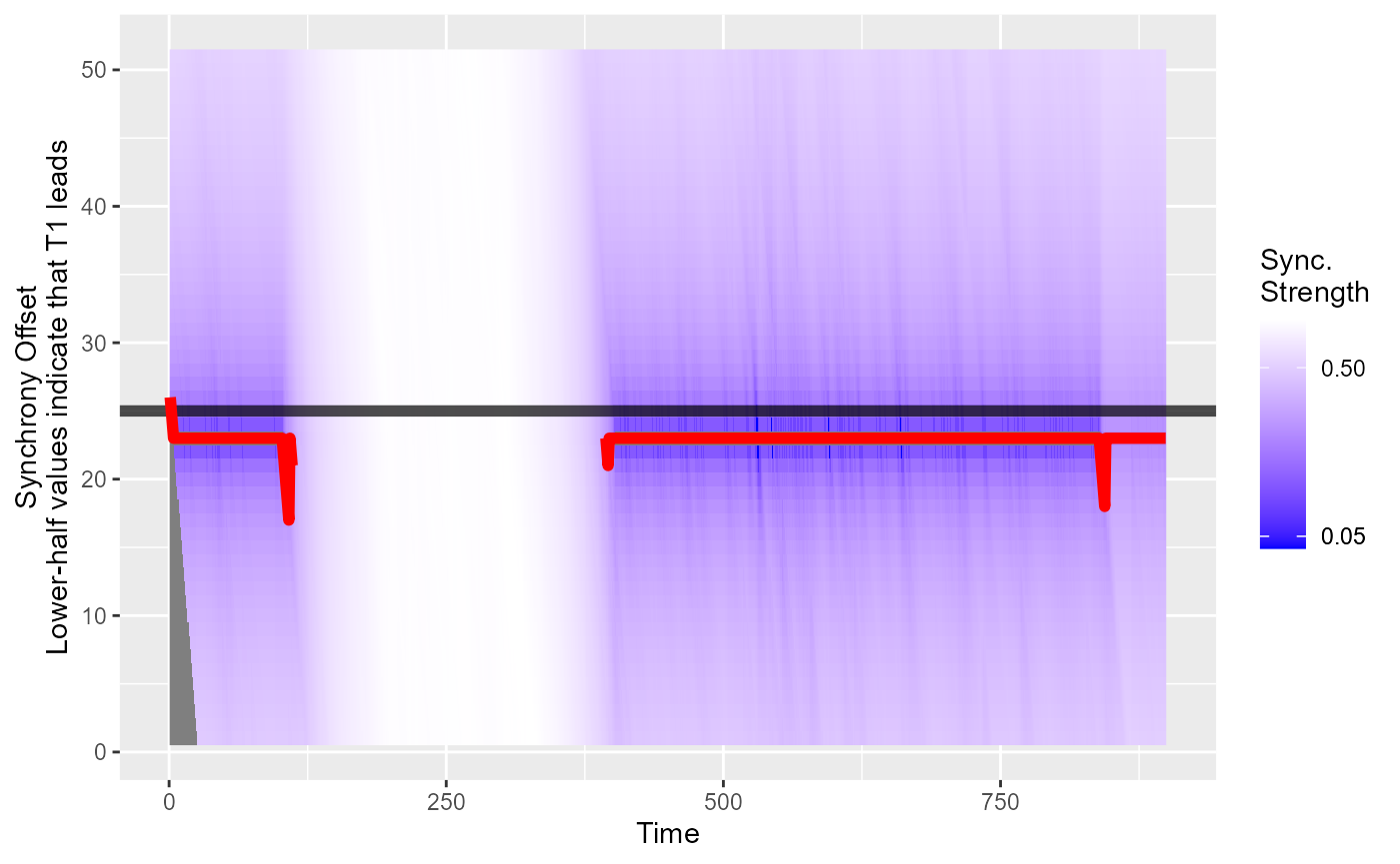
Plot the synchronization profile using the extended plot method:
syncplot(sync)## Don't know how to automatically pick scale for object of type <ts>. Defaulting
## to continuous.## Warning: Transformation introduced infinite values in discrete y-axis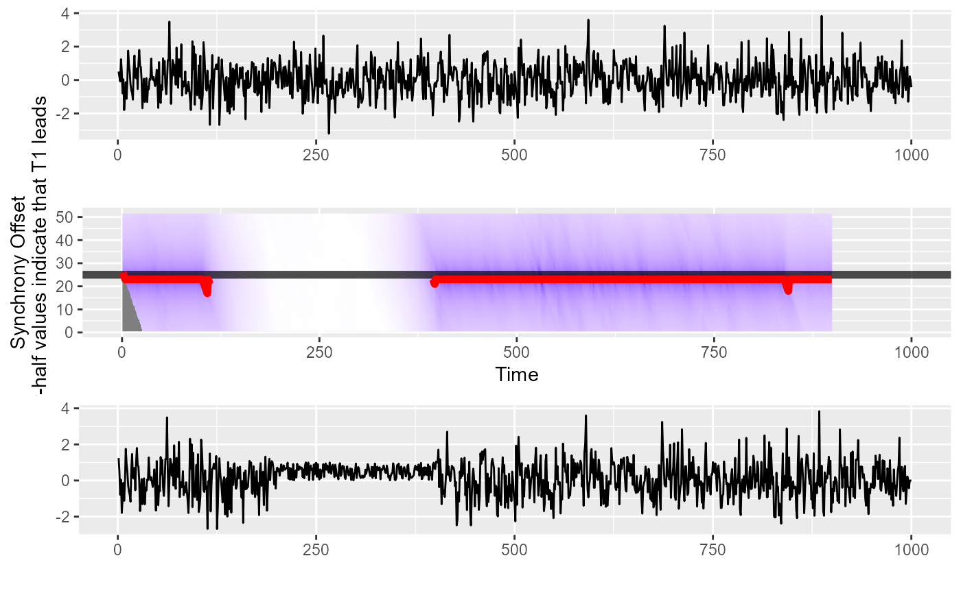
Compute an (experimental) global synchronisation measure (between 0 and 1, with higher values indicating stronger synchrony).
## [1] 0.7419336Now, we further reduce the synchronisation and re-run the algorithm again.
# no synchrony between 200 and 400
t2[200:600] <- runif(201, 0, 1)
## Warning in t2[200:600] <- runif(201, 0, 1): number of items to replace is not a
## multiple of replacement length
sync <- pdcsync(t1, t2)Plot the synchronization profile using the extended plot method:
syncplot(sync)## Don't know how to automatically pick scale for object of type <ts>. Defaulting
## to continuous.## Warning: Transformation introduced infinite values in discrete y-axis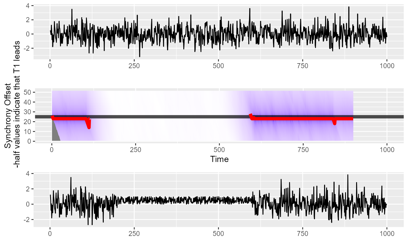
Compute an (experimental) global synchronisation measure (between 0 and 1, with higher values indicating stronger synchrony). This value is lower than before because global synchronisation decreased.
## [1] 0.5348691