Use Case: Linear Regression with Outlier Correction and Bootstrap

Andreas Brandmaier

2025-07-04

This vignette demonstrates how to perform a robust linear regression analysis on the Boston housing data. We start by setting global chunk options and loading the required packages.

library(reproducibleRchunks)
library(MASS)

Load Data

We load the Boston housing data from the MASS package and display the first rows to get an overview of the variables.

boston <- MASS::Boston
knitr::kable(head(boston))

crim	zn	indus	chas	nox	rm	age	dis	rad	tax	ptratio	black	lstat	medv
0.00632	18	2.31	0	0.538	6.575	65.2	4.0900	1	296	15.3	396.90	4.98	24.0
0.02731	0	7.07	0	0.469	6.421	78.9	4.9671	2	242	17.8	396.90	9.14	21.6
0.02729	0	7.07	0	0.469	7.185	61.1	4.9671	2	242	17.8	392.83	4.03	34.7
0.03237	0	2.18	0	0.458	6.998	45.8	6.0622	3	222	18.7	394.63	2.94	33.4
0.06905	0	2.18	0	0.458	7.147	54.2	6.0622	3	222	18.7	396.90	5.33	36.2
0.02985	0	2.18	0	0.458	6.430	58.7	6.0622	3	222	18.7	394.12	5.21	28.7

Code Chunk Reproduction Report

• ✅boston: REPRODUCTION SUCCESSFUL

Outlier Correction

Next, we remove observations with extremely high or low values of medv using the IQR rule to reduce the influence of outliers.

iqr_medv <- IQR(boston$medv)
q <- quantile(boston$medv, c(0.25, 0.75))
lower <- q[1] - 1.5 * iqr_medv
upper <- q[2] + 1.5 * iqr_medv
boston <- boston[boston$medv >= lower & boston$medv <= upper, ]

Code Chunk Reproduction Report

• ✅iqr_medv: REPRODUCTION SUCCESSFUL

• ✅lower: REPRODUCTION SUCCESSFUL

• ✅q: REPRODUCTION SUCCESSFUL

• ✅upper: REPRODUCTION SUCCESSFUL

Linear Regression

We then fit a simple linear regression predicting median house value from the percentage of lower status population (lstat).

model <- lm(medv ~ lstat, data = boston)
summary(model)
#> 
#> Call:
#> lm(formula = medv ~ lstat, data = boston)
#> 
#> Residuals:
#>      Min       1Q   Median       3Q      Max 
#> -12.6960  -2.6909  -0.7157   1.9776  14.6744 
#> 
#> Coefficients:
#>             Estimate Std. Error t value Pr(>|t|)    
#> (Intercept) 30.25803    0.41087   73.64   <2e-16 ***
#> lstat       -0.71853    0.02744  -26.19   <2e-16 ***
#> ---
#> Signif. codes:  0 '***' 0.001 '**' 0.01 '*' 0.05 '.' 0.1 ' ' 1
#> 
#> Residual standard error: 4.103 on 464 degrees of freedom
#> Multiple R-squared:  0.5964, Adjusted R-squared:  0.5956 
#> F-statistic: 685.7 on 1 and 464 DF,  p-value: < 2.2e-16

Code Chunk Reproduction Report

• ✅model: REPRODUCTION SUCCESSFUL

Bootstrap Coefficients

To assess the variability of the coefficients we perform a simple bootstrap. Because analyses based on random numbers lead to different results across runs, we set a random seed to make this step reproducible. See Brandmaier et al. for a detailed discussion of reproducibility and random numbers (https://qcmb.psychopen.eu/index.php/qcmb/article/view/3763/3763.html).

set.seed(123)
boot_coefs <- replicate(1000, {
  idx <- sample(nrow(boston), replace = TRUE)
  coef(lm(medv ~ lstat, data = boston[idx, ]))
})
boot_means <- rowMeans(boot_coefs)
boot_means
#> (Intercept)       lstat 
#>   30.282183   -0.720951

Code Chunk Reproduction Report

• ✅.Random.seed: REPRODUCTION SUCCESSFUL

• ✅boot_coefs: REPRODUCTION SUCCESSFUL

• ✅boot_means: REPRODUCTION SUCCESSFUL

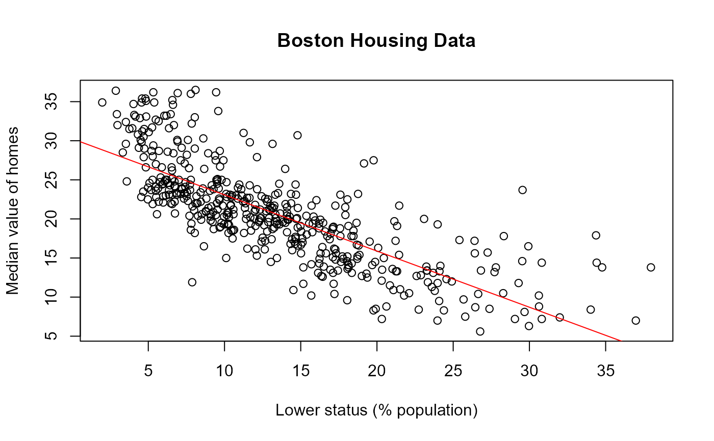
Plot

Finally, we visualise the relation between lstat and medv together with the fitted regression line. Since plots do return objects, they are not tested for reproducibility.

plot(boston$lstat, boston$medv,
     xlab = "Lower status (% population)",
     ylab = "Median value of homes",
     main = "Boston Housing Data")
abline(model, col = "red")

Code Chunk Reproduction Report

No variables were created within this chunk. Cannot generate a reproduction report.