Constraints in semtree
Andreas M. Brandmaier
2026-02-16
Source:vignettes/constraints.Rmd
constraints.RmdConstraints
Load the package
semtree allows different constraints on the split
evaluation (local.invariance, and
focus.parameters). These can be set in the following object
and then passed to the semtree command:
library(semtree)

cnst <- semtree.constraints(local.invariance=NULL,
focus.parameters=NULL)

semtree(model.x, data=df, constraints=cnst)
Simulation
To illustrate the invariance constraints, let’s set up a latent factor model with four indicators and simulate some data with a known predictor structure. Let’s create a dataset as follows:
- a latent construct,
lat, measured by four indicators - two predictors
p1andp2 - only one predictor,
p1, has an mean effect on the latent construct - the other predictor,
p2, has an effect on only one indicator (different loadings across groups; DIF)
N <- 2000
p1 <- sample(size = N,
             x = c(0, 1),
             replace = TRUE)
p2 <- sample(size = N,
             x = c(0, 1),
             replace = TRUE)
lat <- rnorm(N, mean = 0 + p1)
loadings <- c(.5, .8, .7, .9)
observed <- lat %*% t(loadings) + rnorm(N * length(loadings), sd = .1)
observed[, 3] <- observed[, 3] + p2 * 0.5 * lat
cfa.sim <- data.frame(observed, p1 = factor(p1), p2 = factor(p2))
names(cfa.sim)[1:4] <- paste0("x", 1:4)
Here is the OpenMx model specification
require("OpenMx");
manifests<-c("x1","x2","x3","x4")
latents<-c("F")
model.cfa <- mxModel("CFA", type="RAM", manifestVars = manifests,
                     latentVars = latents,
mxPath(from="F",to=c("x1","x2","x3","x4"),
       free=c(TRUE,TRUE,TRUE,TRUE), value=c(1.0,1.0,1.0,1.0) ,
       arrows=1, label=c("F__x1","F__x2","F__x3","F__x4") ),
mxPath(from="one",to=c("x2","x3","x4"),
       free=c(TRUE,TRUE,TRUE), value=c(1.0,1.0,1.0) ,
       arrows=1, label=c("const__x2","const__x3","const__x4") ),
mxPath(from="one",to=c("F"), free=c(TRUE),
       value=c(1.0) , arrows=1, label=c("const__F") ),
mxPath(from="x1",to=c("x1"), free=c(TRUE),
       value=c(1.0) , arrows=2, label=c("VAR_x1") ),
mxPath(from="x2",to=c("x2"), free=c(TRUE),
       value=c(1.0) , arrows=2, label=c("VAR_x2") ),
mxPath(from="x3",to=c("x3"), free=c(TRUE),
       value=c(1.0) , arrows=2, label=c("VAR_x3") ),
mxPath(from="x4",to=c("x4"), free=c(TRUE),
       value=c(1.0) , arrows=2, label=c("VAR_x4") ),
mxPath(from="F",to=c("F"), free=c(FALSE),
       value=c(1.0) , arrows=2, label=c("VAR_F") ),
mxPath(from="one",to=c("x1"), free=F, value=0, arrows=1),
mxData(cfa.sim, type = "raw")
);
Local Invariance
Local invariance builds a tree under which all parameters across the
leafs of a tree may differ but the chosen parameters may not differ
significantly from each other. If they differed significantly, the
respective split is not considered a valid split and is not chosen.
Local constraints are implemented by means of an additional test of
measurement invariance. For each possible split, we fit an additional
null model, in which the locally invariant parameters are constrained to
be equal across the two resulting daughter nodes of a split. Only if we
reject this null hypothesis, we believe that there is measurement
non-invariance and disregard the split. A typical use-case is to the set
of loadings of a factor model as local.invariance to allow
a tree with weakly measurement-invariant leafs.
tree.lc <- semtree(model.cfa, data=cfa.sim, constraints=
                   semtree.constraints(
                     local.invariance= c("F__x1","F__x2","F__x3","F__x4")))
#> > Model was not run. Estimating parameters now.
#> Beginning initial fit attemptFit attempt 0, fit=1298.9451536784, new current best! (was 23577.0760914388)                                                                            > No Invariance alpha selected. alpha.invariance set to:0.05
#> Beginning initial fit attempt                             Beginning initial fit attemptFit attempt 0, fit=-1283.02560315233, new current best! (was 621.360407936133)                                                                              Beginning initial fit attemptFit attempt 0, fit=-790.650598262703, new current best! (was -667.657401072649)                                                                               Beginning initial fit attemptFit attempt 0, fit=-736.010057168879, new current best! (was -615.36820207966)                                                                              Beginning initial fit attemptFit attempt 0, fit=-1332.12327007281, new current best! (was 677.584745742238)                                                                              Beginning initial fit attemptFit attempt 0, fit=-795.443714634396, new current best! (was -676.959406258319)                                                                               Beginning initial fit attemptFit attempt 0, fit=-784.971830514303, new current best! (was -655.163863814537)                                                                               ✔ Tree construction finished [took 3s].
Now we find p1 as the only predictor that yields
subgroups that pass the measurement invariance test. Even though we have
chosen the four factor loadings as local.invariance
constraint, they are allowed to differ numerically but there was no
significant difference between them.
plot(tree.lc)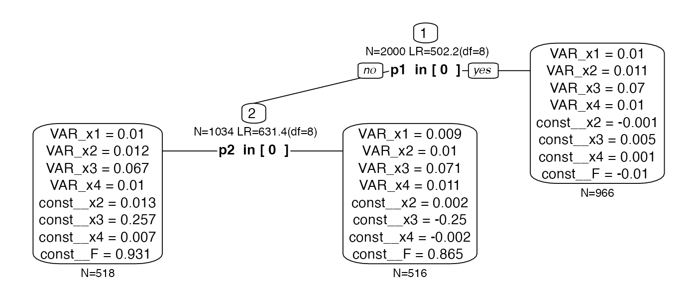
Focus Parameters
First, we create some data. Here, we generate 1,000 bivariate
observations x1 and x2 gathered in a data
frame called obs. Also, there are two predictors
grp1 and grp2. Predictor grp1
predicts a mean difference in x1 whereas grp2
predicts differences only in x2.
set.seed(123)
N <- 1000
grp1 <- sample(x = c(0,1), size=N, replace=TRUE)
grp2 <- sample(x = c(0,1), size=N, replace=TRUE)
Sigma <- matrix(byrow=TRUE,
                        nrow=2,c(2,0.2,
                                0.2,1))
obs <- MASS::mvrnorm(N,mu=c(0,0),
                      Sigma=Sigma)
obs[,1] <- obs[,1] + ifelse(grp1,3,0)
obs[,2] <- obs[,2] + ifelse(grp2,3,0)
df.biv <- data.frame(obs, grp1=factor(grp1), grp2=factor(grp2))
names(df.biv)[1:2] <- paste0("x",1:2)
A tree without constraints should recover both parameters (given
large enough sample and effect sizes) because it explores differences in
both means and covariance structure of x1 and
x2. Here is an OpenMx model specification for a saturated
bivariate model:
manifests<-c("x1","x2")
model.biv <- mxModel("Bivariate_Model",
type="RAM",
manifestVars = manifests,
latentVars = c(),
mxPath(from="x1",to=c("x1","x2"),
       free=c(TRUE,TRUE), value=c(1.0,.2) ,
       arrows=2, label=c("VAR_x1","COV_x1_x2") ),
mxPath(from="x2",to=c("x2"), free=c(TRUE),
       value=c(1.0) , arrows=2, label=c("VAR_x2") ),
mxPath(from="one",to=c("x1","x2"), label=c("mu1","mu2"),
       free=TRUE, value=0, arrows=1),
mxData(df.biv, type = "raw")
);
Let’s run this model in OpenMx:
result <- mxRun(model.biv)
#> Running Bivariate_Model with 5 parameters
summary(result)
#> Summary of Bivariate_Model
#>
#> free parameters:
#>        name matrix row col  Estimate  Std.Error A
#> 1    VAR_x1      S  x1  x1 4.0283800 0.18015402
#> 2 COV_x1_x2      S  x1  x2 0.3039196 0.11443875
#> 3    VAR_x2      S  x2  x2 3.2282345 0.14437018
#> 4       mu1      M   1  x1 1.4187341 0.06346925
#> 5       mu2      M   1  x2 1.4628999 0.05681735
#>
#> Model Statistics:
#>                |  Parameters  |  Degrees of Freedom  |  Fit (-2lnL units)
#>        Model:              5                   1995              8233.926
#>    Saturated:              5                   1995                    NA
#> Independence:              4                   1996                    NA
#> Number of observations/statistics: 1000/2000
#>
#> Information Criteria:
#>       |  df Penalty  |  Parameters Penalty  |  Sample-Size Adjusted
#> AIC:       4243.926               8243.926                 8243.986
#> BIC:      -5547.046               8268.465                 8252.584
#> To get additional fit indices, see help(mxRefModels)
#> timestamp: 2026-02-16 15:35:08
#> Wall clock time: 0.0235641 secs
#> optimizer:  SLSQP
#> OpenMx version number: 2.22.9
#> Need help?  See help(mxSummary)
Now, we grow a tree without constraints:
tree.biv <- semtree(model.biv, data=df.biv)
#> > Model was not run. Estimating parameters now.
#> Beginning initial fit attemptFit attempt 0, fit=8233.92582585158, new current best! (was 14528.4141425595)                                                                             Beginning initial fit attemptFit attempt 0, fit=8233.92582585143, new current best! (was 8233.92582585158)                                                                             Beginning initial fit attemptFit attempt 0, fit=3454.12434636158, new current best! (was 4066.88531956853)                                                                             Beginning initial fit attemptFit attempt 0, fit=1555.54412300078, new current best! (was 1720.05414323717)                                                                             Beginning initial fit attemptFit attempt 0, fit=1569.26472590267, new current best! (was 1734.07020312441)                                                                             Beginning initial fit attemptFit attempt 0, fit=3566.5692080098, new current best! (was 4167.0405062829)                                                                           Beginning initial fit attemptFit attempt 0, fit=1593.91684303245, new current best! (was 1780.60715329424)                                                                             Beginning initial fit attemptFit attempt 0, fit=1576.27862642528, new current best! (was 1785.96205471556)                                                                             ✔ Tree construction finished [took 2s].
As expected, we obtain a tree structure that has both p1
and p2 (here we use the viridis colors to give each leaf
node a different frame color, which we’ll use later again):
# default white color for all nodes
cols <- rep("black", semtree:::getNumNodes(tree.biv))
cols[as.numeric(row.names(semtree:::getTerminalNodes(tree.biv)))] <- viridis:::viridis_pal()(4)

plot(tree.biv, border.col=cols)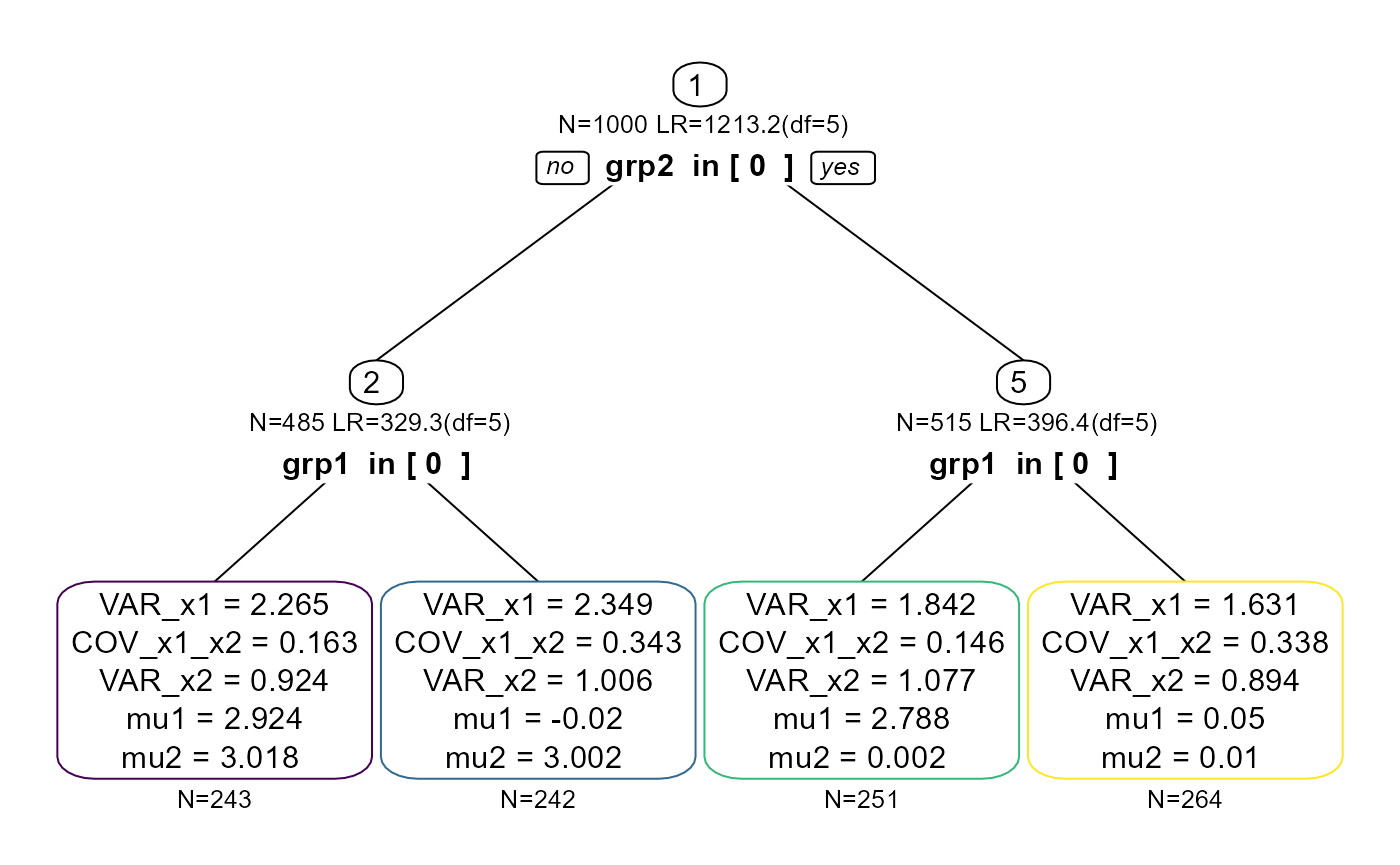
Let us visualize what this tree is doing. Here is the empirical joint
distribution of both x1 and x2:
require("ggplot2")
ggplot(data = df.biv, aes(x=x1, y=x2))+
  geom_density_2d()+
  theme_classic()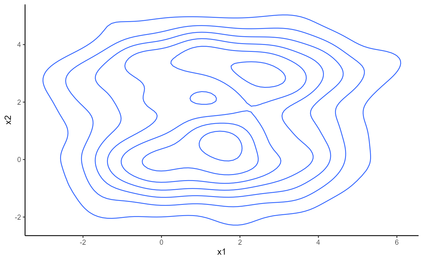
And here is the partition of the observed two-dimensional space implied by the leafs of the tree (compare the density colors to the colors of the leaf nodes in the earlier dendrogram):
df.biv.pred <- data.frame(df.biv,
  leaf=factor(getLeafs(tree=tree.biv, data = df.biv)))
ggplot(data = df.biv.pred, aes(x=x1, y=x2))+
  geom_density_2d(aes(colour=leaf))+
  viridis::scale_color_viridis(discrete=TRUE)+
  theme_classic()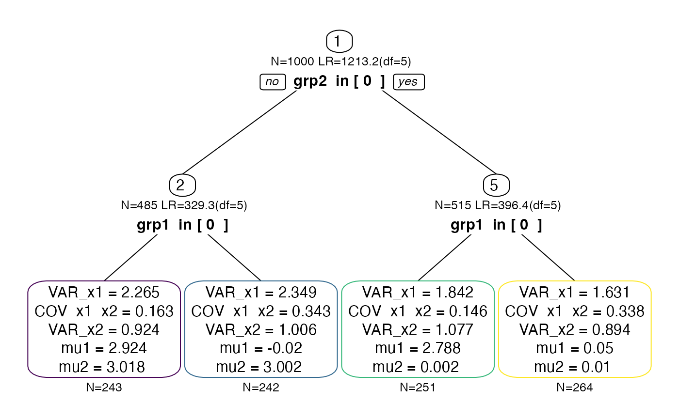
What if we were interested only in splits with respect to one of the
two dimensions? In this case, we can set a focus.parameter.
Focus parameters change the split evaluation such that only splits are
evaluated that maximize the misfit between a model in which all
parameters are free and a model in which all parameters are free but the
parameters given in focus.parameter.
Let us first set mu1 as focus parameter:
tree.biv2 <- semtree(model.biv, df.biv, constraints=
                      semtree.constraints(focus.parameters = "mu1"))
#> > Model was not run. Estimating parameters now.
#> Beginning initial fit attemptFit attempt 0, fit=8233.92582585158, new current best! (was 14528.4141425595)                                                                             Beginning initial fit attemptFit attempt 0, fit=8233.92582585143, new current best! (was 8233.92582585158)                                                                             Beginning initial fit attemptFit attempt 0, fit=3740.92185296731, new current best! (was 4086.36288912548)                                                                             Beginning initial fit attemptFit attempt 0, fit=3795.16307144921, new current best! (was 4147.56293672595)                                                                             ✔ Tree construction finished [took 1s].
plot(tree.biv2)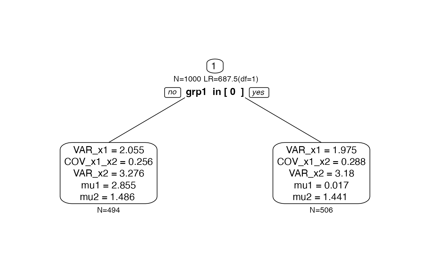
As expected, the resulting tree structure only has grp1
as predictor because grp1 predicts differences in
mu1. Predictor grp2 did not come up anymore.
Now, if we set mu2, we should see the exact opposite
picture:
tree.biv3 <- semtree(model.biv, df.biv, constraints=
                      semtree.constraints(focus.parameters = "mu2"))
#> > Model was not run. Estimating parameters now.
#> Beginning initial fit attemptFit attempt 0, fit=8233.92582585158, new current best! (was 14528.4141425595)                                                                             Beginning initial fit attemptFit attempt 0, fit=8233.92582585143, new current best! (was 8233.92582585158)                                                                             Beginning initial fit attemptFit attempt 0, fit=3454.12434636158, new current best! (was 4066.88531956853)                                                                             Beginning initial fit attemptFit attempt 0, fit=3566.5692080098, new current best! (was 4167.0405062829)                                                                           ✔ Tree construction finished [took 1s].
And, indeed, we see only grp2 as predictor whereas
grp1 was not selected this time.
plot(tree.biv3)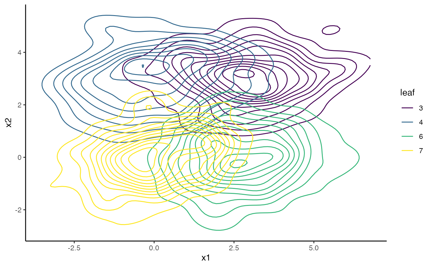
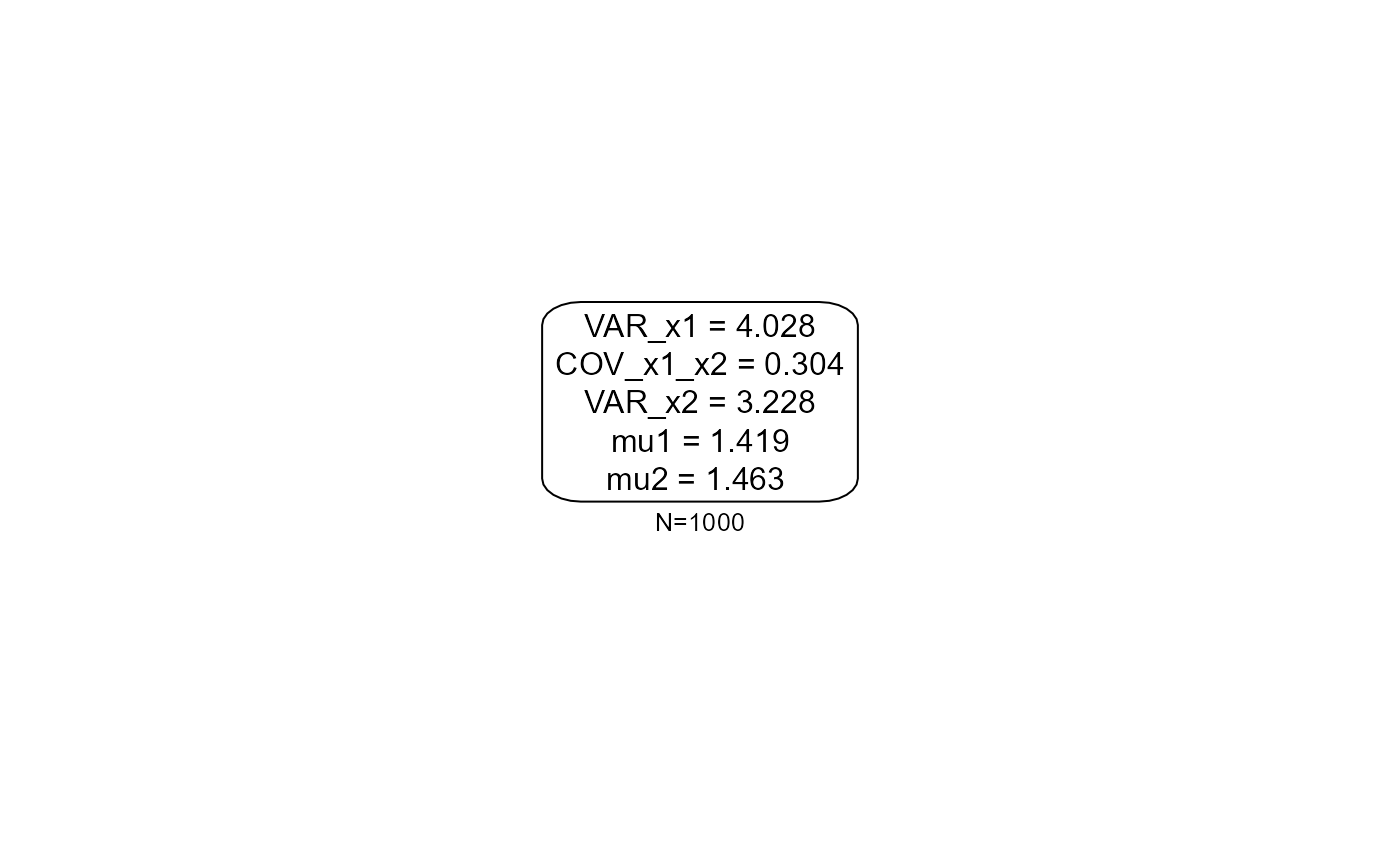
Finally, we set the focus.parameter to one of the
variance parameters. None of the predictors predicts differences in the
variance, so we expect an empty tree (only the root node; no predictors
selected):
tree.biv4 <- semtree(model.biv, df.biv, constraints=
                      semtree.constraints(focus.parameters = "VAR_x2"))
#> > Model was not run. Estimating parameters now.
#> Beginning initial fit attemptFit attempt 0, fit=8233.92582585158, new current best! (was 14528.4141425595)                                                                             Beginning initial fit attemptFit attempt 0, fit=8233.92582585143, new current best! (was 8233.92582585158)                                                                             ✔ Tree construction finished [took less than a second].

plot(tree.biv4)