Focus parameters in SEM forests

We first generate a mixture of bivariate normal distributions. The distributions differ only by their x- and y-displacement, that is, by their mean values. There are two predictors grp1 and grp2 which predict the differences in means. grp1 predicts differences in the first dimension and grp2 predicts differences in the second dimension. Without focus parameter, both predictors are needed to distinguish all four groups. If one of the two means is chosen as a focus parameter, only one of the two predictors is important.


library(semtree)
#> Loading required package: OpenMx
#> OpenMx may run faster if it is compiled to take advantage of multiple cores.
set.seed(123)
N <- 1000
grp1 <- factor(sample(x = c(0,1), size=N, replace=TRUE))
grp2 <- factor(sample(x = c(0,1), size=N, replace=TRUE))
noise <- factor(sample(x = c(0,1),size=N, replace=TRUE))
Sigma <- matrix(byrow=TRUE,
                nrow=2,c(2,0.2,
                         0.2,1))
obs <- MASS::mvrnorm(N,mu=c(0,0),
                     Sigma=Sigma)
obs[,1] <- obs[,1] + ifelse(grp1==1,3,0)
obs[,2] <- obs[,2] + ifelse(grp2==1,3,0)
df.biv <- data.frame(obs, grp1, grp2, noise)
names(df.biv)[1:2] <- paste0("x",1:2)
manifests<-c("x1","x2")

The following code specifies a bivariate Gaussian model with five parameters:

model.biv <- mxModel("Bivariate_Model", 
                     type="RAM",
                     manifestVars = manifests,
                     latentVars = c(),
                     mxPath(from="x1",to=c("x1","x2"), 
                            free=c(TRUE,TRUE), value=c(1.0,.2) , 
                            arrows=2, label=c("VAR_x1","COV_x1_x2") ),
                     mxPath(from="x2",to=c("x2"), free=c(TRUE), 
                            value=c(1.0) , arrows=2, label=c("VAR_x2") ),
                     mxPath(from="one",to=c("x1","x2"), label=c("mu1","mu2"),
                            free=TRUE, value=0, arrows=1),
                     mxData(df.biv, type = "raw")
);
result <- mxRun(model.biv)
#> Running Bivariate_Model with 5 parameters
summary(result)
#> Summary of Bivariate_Model 
#>  
#> free parameters:
#>        name matrix row col  Estimate  Std.Error A
#> 1    VAR_x1      S  x1  x1 4.0583666 0.18149573  
#> 2 COV_x1_x2      S  x1  x2 0.1970528 0.11384948  
#> 3    VAR_x2      S  x2  x2 3.1848900 0.14243161  
#> 4       mu1      M   1  x1 1.4858354 0.06370544  
#> 5       mu2      M   1  x2 1.4551364 0.05643474  
#> 
#> Model Statistics: 
#>                |  Parameters  |  Degrees of Freedom  |  Fit (-2lnL units)
#>        Model:              5                   1995              8231.944
#>    Saturated:              5                   1995                    NA
#> Independence:              4                   1996                    NA
#> Number of observations/statistics: 1000/2000
#> 
#> Information Criteria: 
#>       |  df Penalty  |  Parameters Penalty  |  Sample-Size Adjusted
#> AIC:       4241.944               8241.944                 8242.004
#> BIC:      -5549.028               8266.483                 8250.602
#> CFI: NA 
#> TLI: 1   (also known as NNFI) 
#> RMSEA:  0  [95% CI (NA, NA)]
#> Prob(RMSEA <= 0.05): NA
#> To get additional fit indices, see help(mxRefModels)
#> timestamp: 2024-04-15 22:33:42 
#> Wall clock time: 0.02595901 secs 
#> optimizer:  SLSQP 
#> OpenMx version number: 2.21.1 
#> Need help?  See help(mxSummary)

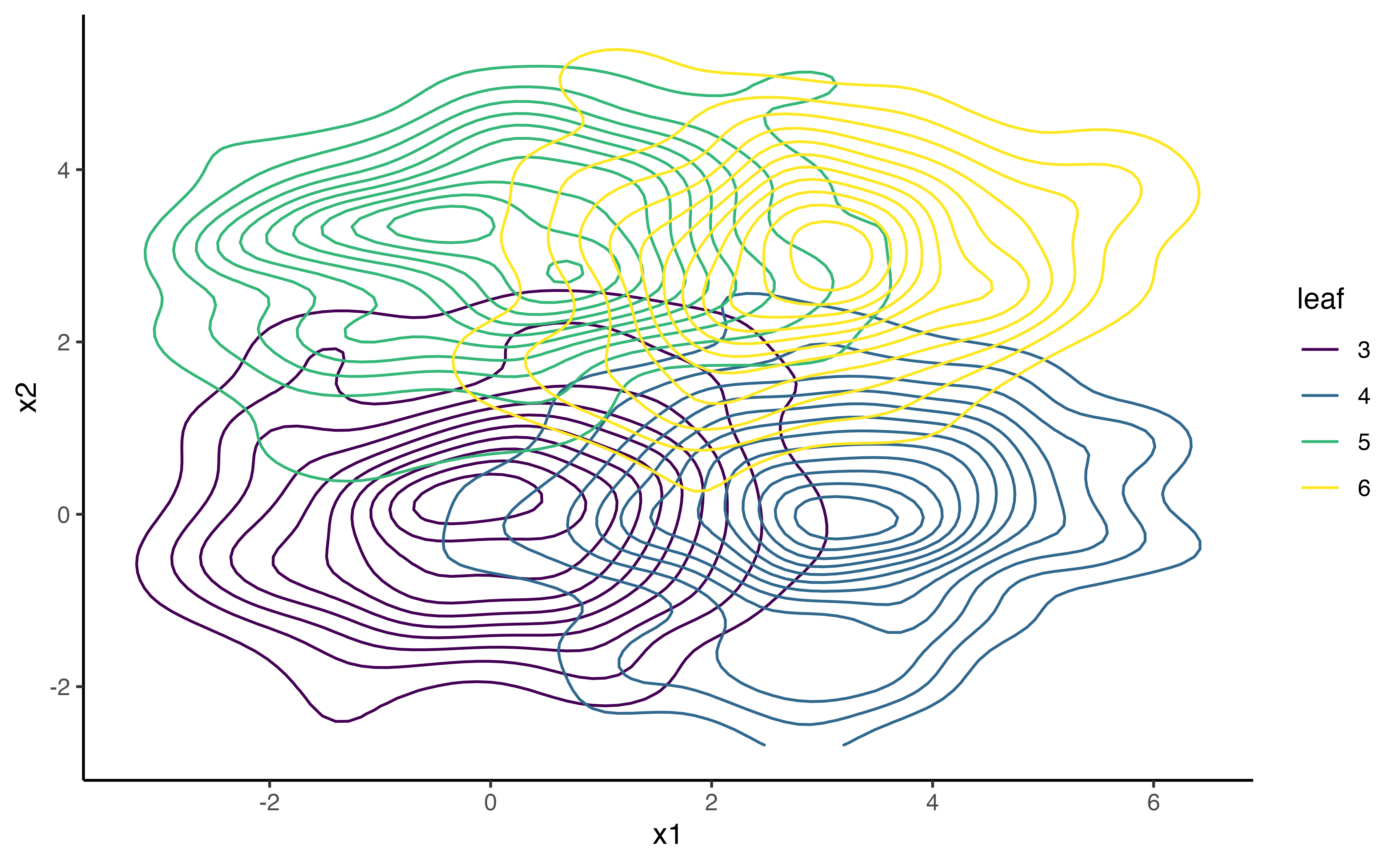
This is how the data look in a 2D space:

df.biv.pred <- data.frame(df.biv, 
  leaf=factor(as.numeric(df.biv$grp2)*2+as.numeric(df.biv$grp1)))
  ggplot(data = df.biv.pred, aes(x=x1, y=x2, group=leaf))+ 
  geom_density_2d(aes(colour=leaf))+ 
  viridis::scale_color_viridis(discrete=TRUE)+
  theme_classic()

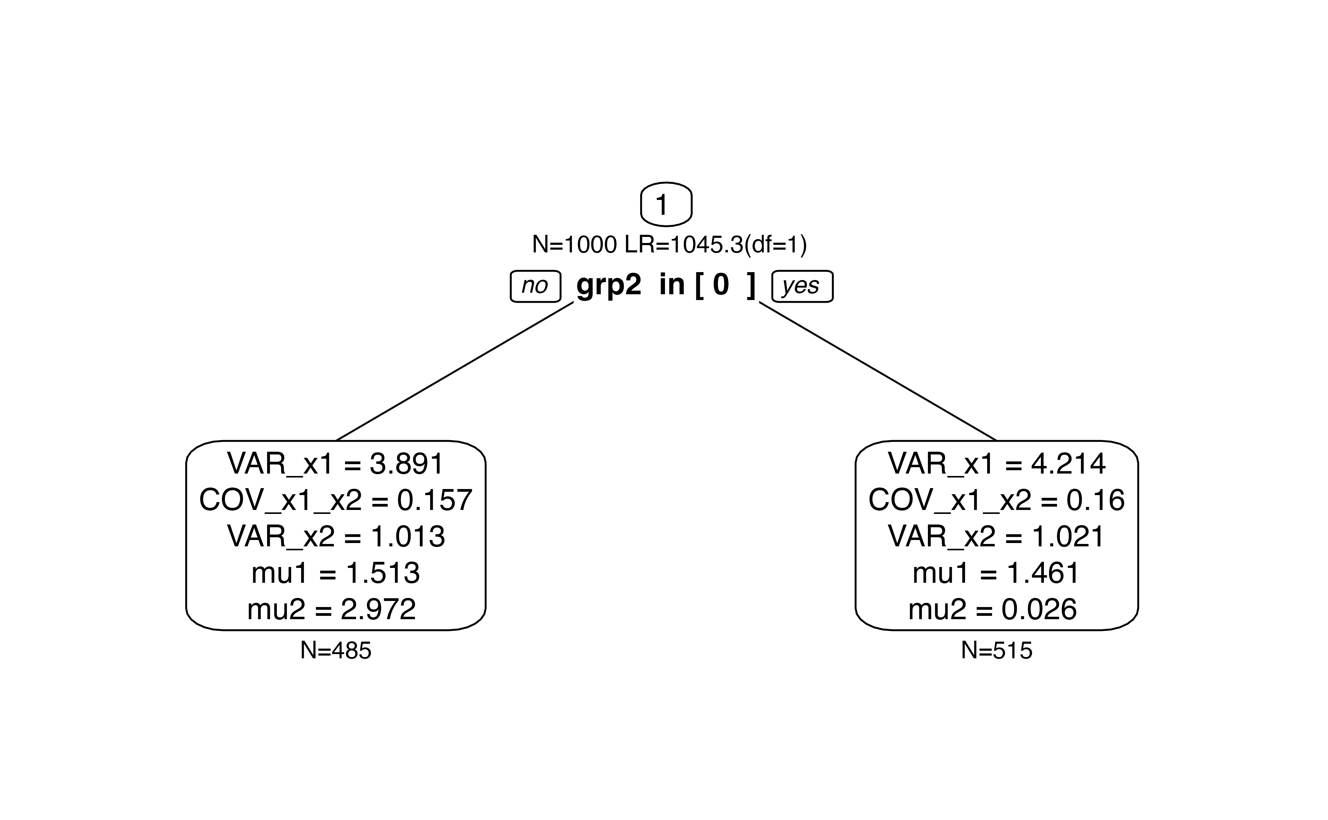
Now, we choose the mean of the second dimension mu2 as focus parameter. We expect that only predictor grp2. This is what we see in a single tree.

fp <- "mu2" # predicted by grp2
#fp <- "mu1" # predicted by grp1

tree.biv <- semtree(model.biv, data=df.biv, constraints = list(focus.parameters=fp))

plot(tree.biv)

Now, we are repeating the same analysis in a forest.

forest <- semforest(model.biv, data=df.biv,
                    constraints = list(focus.parameters=fp),
                    control=semforest.control(num.trees=10, control=semtree.control(method="score",alpha=1)))

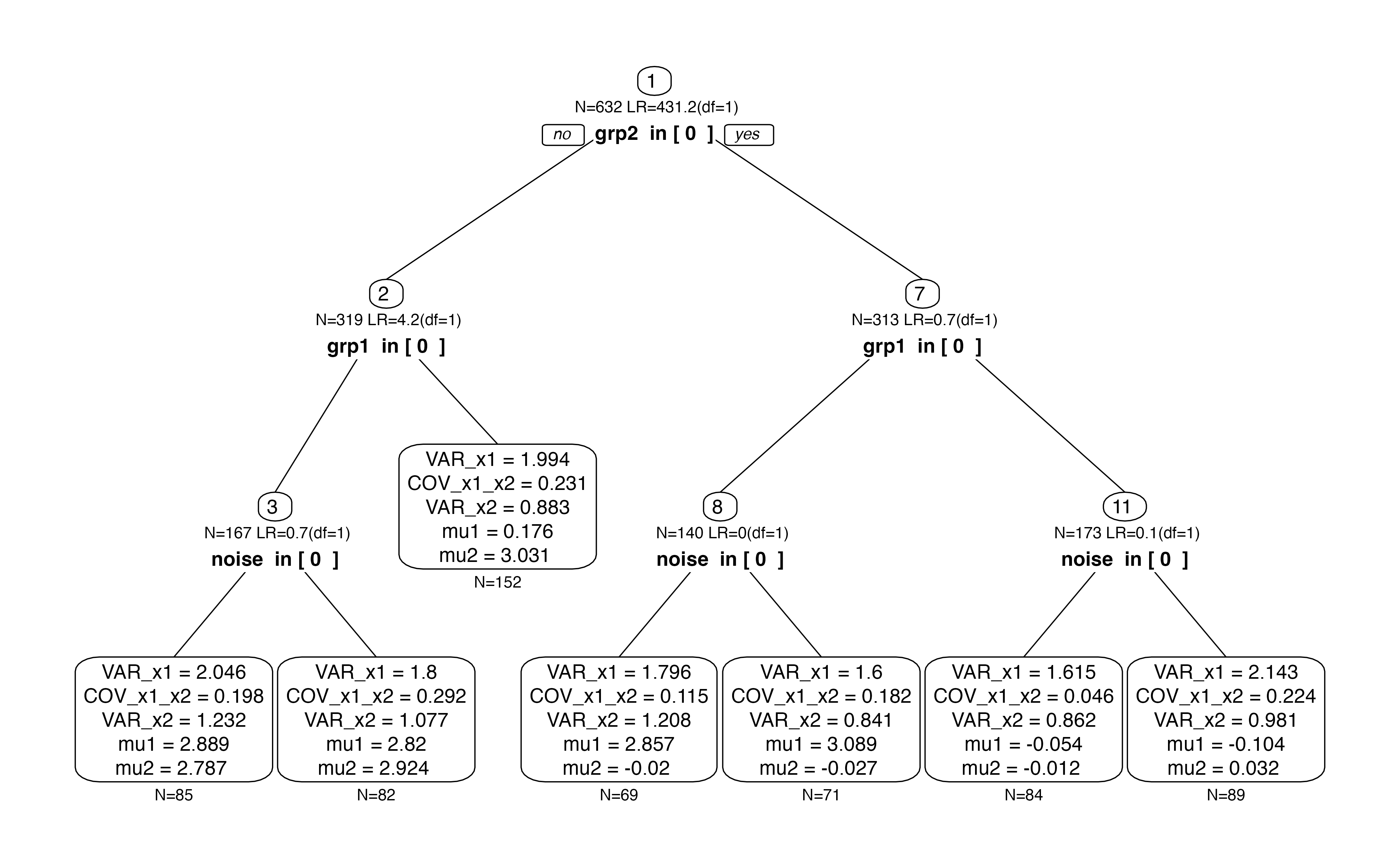
By default, we see that individual trees are fully grown (without a p-value threshold). The first split is according to grp2 because it best explains the group differences. Subsequent splits are according to grp1 even though the chi2 values are close to zero. They only appear because there is no p-value-based stopping criterion.

plot(forest$forest[[1]])

Now, let us investigate the permutation-based variable importance:


vim <- varimp(forest, method="permutationFocus")

plot(vim, main="Variable Importance")

Andreas M. Brandmaier

2024-04-15