SEM Trees with score-based tests

In this example, we will explore how score-based SEM trees can be used. Score-based tests for variable and split-point selection are preferable because they are fast to compute, perform unbiased variable selection, and have better statistical power than some other selection algorithms proposed earlier.

For this illustration, we will use the affect dataset and a simple (non-latent) SEM, which just has one observed variable. Using such a simple model is similar to using a conventional decision tree or random forest; however, the SEM tree version not only finds differences in the mean prediction across leafs but also in the variances (ie., individual differences) of the criterion variable.

Load data

Load affect dataset from the psychTools package. These are data from two studies conducted in the Personality, Motivation and Cognition Laboratory at Northwestern University to study affect dimensionality and the relationship to various personality dimensions. In the following code, we replace the numeric film labels with the movie titles. Also, we select a subset of predictors including the film, personality dimensions, trait anxiety and affect before having watched the movie.

library(psychTools)
data(affect)

affect$Film <- factor(affect$Film, ordered = FALSE, 
                      labels=c("Frontline", "Halloween", "Nat. Geographic","Parenthood"))


tree.data <- affect[,c("Film","neur","ext","soc","traitanx","NA1","PA1")] 
tree.data$DeltaPA <- affect$PA2-affect$PA1

knitr::kable(head(tree.data))

Film	neur	ext	soc	traitanx	NA1	PA1	DeltaPA
Nat. Geographic	9	18	10	24	2	26	-19
Nat. Geographic	12	16	8	41	4	10	-5
Nat. Geographic	5	6	1	37	2	4	-1
Nat. Geographic	15	12	6	54	0	1	-1
Nat. Geographic	2	14	6	39	13	7	9
Frontline	15	6	4	51	1	5	-3

Create simple model of state anxiety

Here, we create a simple SEM with a single observed variable. No latent variables - only two parameters: mean of DeltaPA and variance of DeltaPA.

library(OpenMx)
#> OpenMx may run faster if it is compiled to take advantage of multiple cores.
manifests<-c("DeltaPA")
latents<-c()
model <- mxModel("Simple Model", 
type="RAM",
manifestVars = manifests,
latentVars = latents,
mxPath(from="one",to=manifests, free=c(TRUE), value=c(1.0) , arrows=1, label=c("mu") ),
mxPath(from=manifests,to=manifests, free=c(TRUE), value=c(1.0) , arrows=2, label=c("sigma2") ),
mxData(tree.data, type = "raw")
);

result <- mxRun(model)
#> Running Simple Model with 2 parameters
summary(result)
#> Summary of Simple Model 
#>  
#> free parameters:
#>     name matrix     row     col    Estimate Std.Error A
#> 1 sigma2      S DeltaPA DeltaPA 27.90300741 2.1722417  
#> 2     mu      M       1 DeltaPA  0.09514715 0.2907414 !
#> 
#> Model Statistics: 
#>                |  Parameters  |  Degrees of Freedom  |  Fit (-2lnL units)
#>        Model:              2                    328              2034.982
#>    Saturated:              2                    328                    NA
#> Independence:              2                    328                    NA
#> Number of observations/statistics: 330/330
#> 
#> Information Criteria: 
#>       |  df Penalty  |  Parameters Penalty  |  Sample-Size Adjusted
#> AIC:      1378.9818               2038.982                 2039.018
#> BIC:       132.8794               2046.580                 2040.236
#> CFI: NA 
#> TLI: 1   (also known as NNFI) 
#> RMSEA:  0  [95% CI (NA, NA)]
#> Prob(RMSEA <= 0.05): NA
#> To get additional fit indices, see help(mxRefModels)
#> timestamp: 2024-04-15 22:33:34 
#> Wall clock time: 0.02639604 secs 
#> optimizer:  SLSQP 
#> OpenMx version number: 2.21.1 
#> Need help?  See help(mxSummary)

Score-based Tests

Use score-based tests to create the tree. Use Bonferroni-correction to adjust for multiple testing of predictors.

library(semtree)
ctrl = semtree.control(
  method="score", 
  bonferroni = TRUE)

tree = semtree( model = result, 
                data = tree.data, 
                control=ctrl)

Now let us plot the tree.

plot(tree)

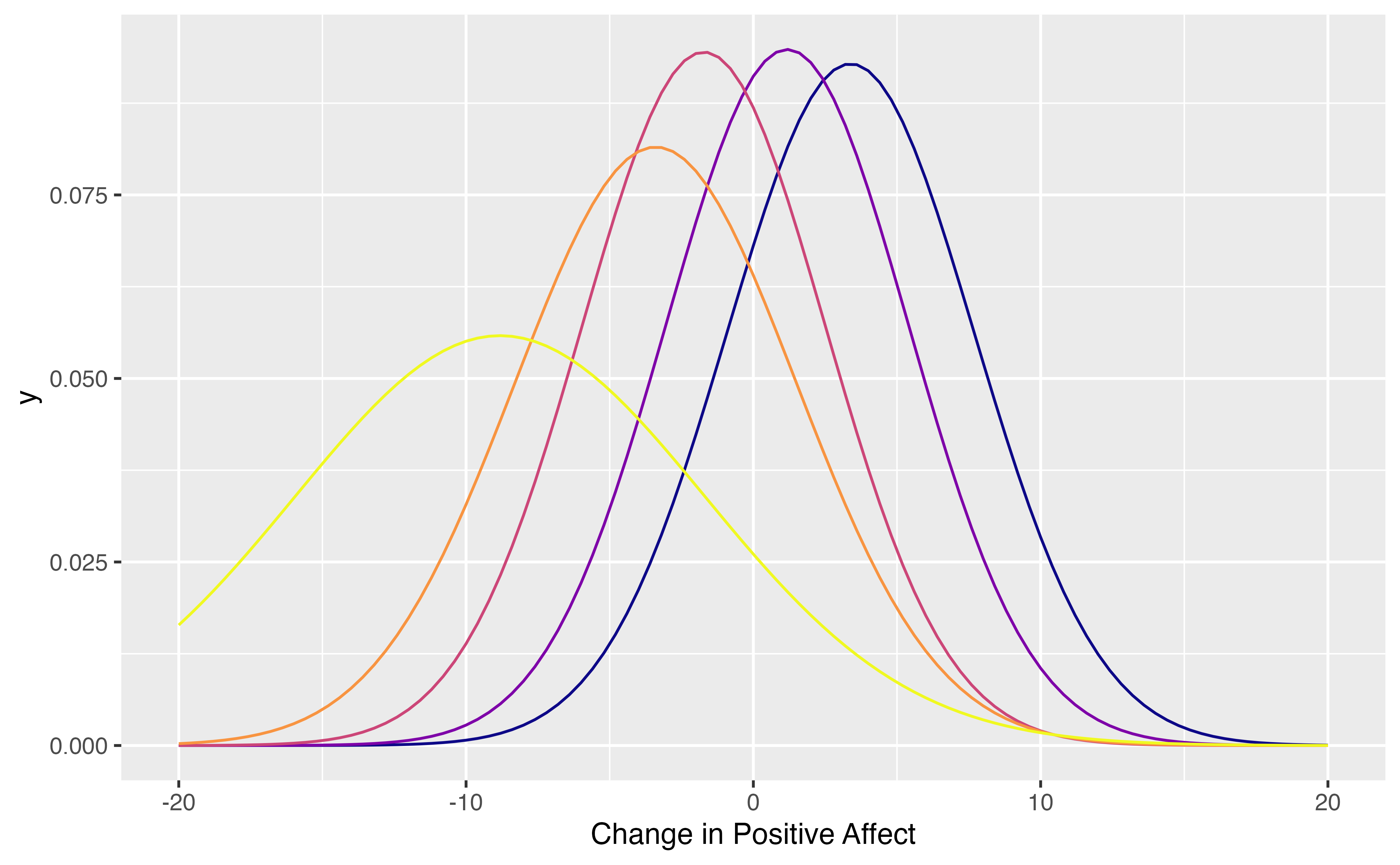
Implied mixture model:

tndata <- semtree::getTerminalNodes(tree)

cols <- viridis::plasma(nrow(tndata))

pl <- ggplot2::ggplot(data = data.frame(x = c(-20, 20)), ggplot2::aes(x))+
  ggplot2::xlab("Change in Positive Affect")

for (i in 1:nrow(tndata)) {
  pl <- pl + ggplot2::stat_function(fun = dnorm, 
      n = 101, col=cols[i], args = list(mean = tndata[i,2], sd = sqrt(tndata[i,1])))
}

plot(pl)

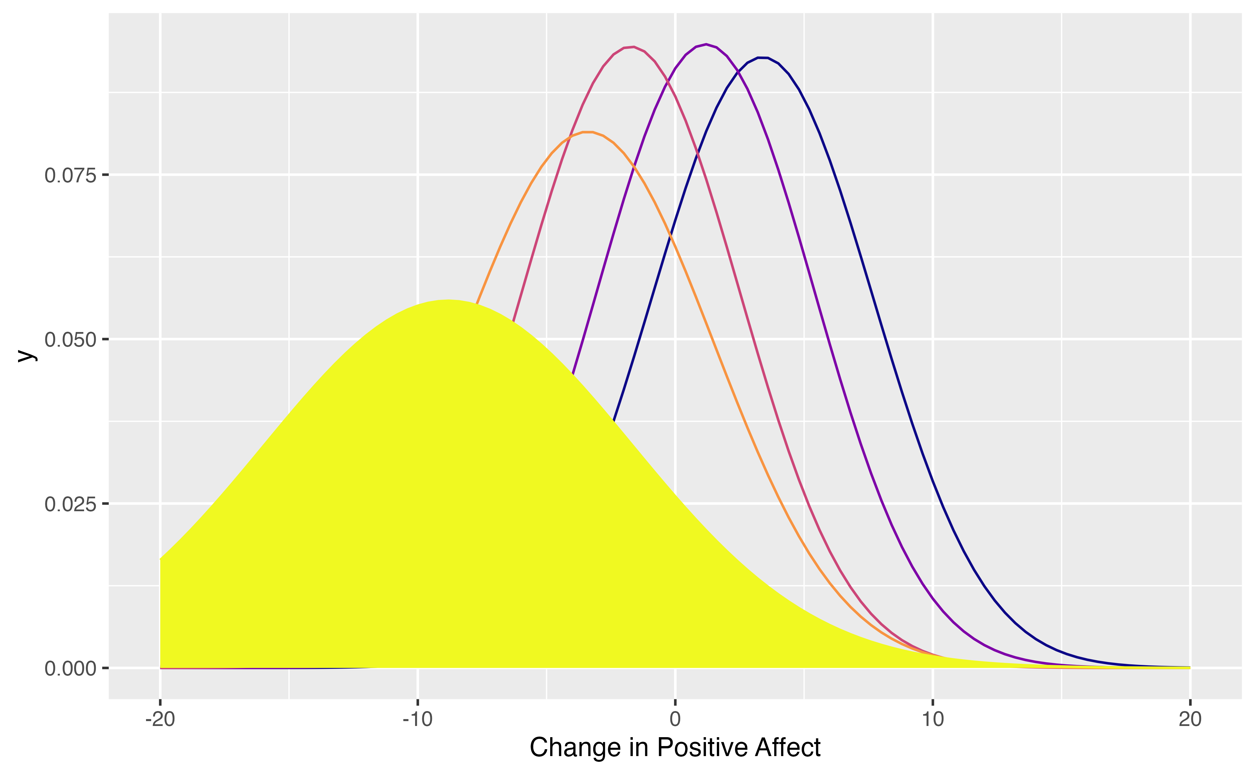
Let us inspect the group with the largest negative change. This is the group of participants, who started out with a high positive affect and then had to watch a war movie.

i <- which.min(tndata$mu)

pl <- pl +ggplot2::geom_area(stat = "function", 
                             fun = function(x){dnorm(x,mean=tndata[i,2],sd=sqrt(tndata[i,1]))}, 
                             fill = cols[i])+
      ggplot2::geom_label(x=-10,y=.12, label="People with very high positive \naffect, which then watched\n a war film")

plot(pl)

Andreas M. Brandmaier

2024-04-15

Load data

Create simple model of state anxiety

Score-based Tests