SEM Forests

This example demonstrates how SEM forests can be grown. SEM forests are ensembles of typically hundreds to thousands of SEM trees. Using permutation-based variable importance estimates, we can aggregate the importance of each predictor for improving model fit.

Here, we use the affect dataset and a simple SEM with only a single observed variable and no latent variables.

Load data

Load affect dataset from the psychTools package. These are data from two studies conducted in the Personality, Motivation and Cognition Laboratory at Northwestern University to study affect dimensionality and the relationship to various personality dimensions.

library(psychTools)
data(affect)

affect <- affect[complete.cases(affect$state2), ]
affect$BDI <- NULL # Drop affect because it is NA
affect$Study <- NULL # Drop Study because it is constant

knitr::kable(head(affect))

	Film	ext	neur	imp	soc	lie	traitanx	state1	EA1	TA1	PA1	NA1	EA2	TA2	PA2	NA2	state2	MEQ
161	4	7	19	5	2	3	60	45	2.0	14	2	2	3	15	3.0	0	48	49
162	1	10	16	3	4	1	52	53	3.0	18	0	3	7	17	0.0	2	55	43
163	1	11	7	2	9	3	39	27	21.0	11	18	1	23	21	14.5	15	51	50
164	1	10	22	4	4	1	53	68	7.0	22	6	14	14	21	12.0	20	71	49
165	1	8	6	1	7	2	38	38	4.0	8	3	0	2	8	0.0	3	35	39
166	4	17	14	6	10	1	50	51	1.3	9	0	9	0	17	0.0	0	37	21


affect$Film <- as.factor(affect$Film)
affect$lie <- as.ordered(affect$lie)
affect$imp <- as.ordered(affect$imp)

Create simple model of state anxiety

The following code implements a simple SEM with only a single manifest variables and two parameters, the mean of state anxiety after having watched a movie (state2), $\mu$ , and the variance of state anxiety, $\sigma^2$ .

library(OpenMx)
manifests<-c("state2")
latents<-c()
model <- mxModel("Univariate Normal Model", 
type="RAM",
manifestVars = manifests,
latentVars = latents,
mxPath(from="one",to=manifests, free=c(TRUE), 
       value=c(50.0) , arrows=1, label=c("mu") ),
mxPath(from=manifests,to=manifests, free=c(TRUE), 
       value=c(100.0) , arrows=2, label=c("sigma2") ),
mxData(affect, type = "raw")
);

result <- mxRun(model)
#> Running Univariate Normal Model with 2 parameters

These are the estimates of the model when run on the entire sample:

summary(result)
#> Summary of Univariate Normal Model 
#>  
#> free parameters:
#>     name matrix    row    col  Estimate  Std.Error A
#> 1 sigma2      S state2 state2 115.05414 12.4793862  
#> 2     mu      M      1 state2  42.45118  0.8226717  
#> 
#> Model Statistics: 
#>                |  Parameters  |  Degrees of Freedom  |  Fit (-2lnL units)
#>        Model:              2                    168              1289.158
#>    Saturated:              2                    168                    NA
#> Independence:              2                    168                    NA
#> Number of observations/statistics: 170/170
#> 
#> Information Criteria: 
#>       |  df Penalty  |  Parameters Penalty  |  Sample-Size Adjusted
#> AIC:       953.1576               1293.158                 1293.229
#> BIC:       426.3434               1299.429                 1293.096
#> To get additional fit indices, see help(mxRefModels)
#> timestamp: 2026-01-23 13:22:57 
#> Wall clock time: 0.05539393 secs 
#> optimizer:  SLSQP 
#> OpenMx version number: 2.22.9 
#> Need help?  See help(mxSummary)

Forest

Create a forest control object that stores all tuning parameters of the forest. Note that we use only 5 trees for illustration. Please increase the number in real applications to several hundreds. To speed up computation time, consider score-based test for variable selection in the trees.

control <- semforest_score_control(num.trees = 50)
print(control)
#> SEM-Forest control:
#> -----------------
#> Number of Trees:  50 
#> Sampling:  subsample 
#> Comparisons per Node: 2 
#> 
#>  SEM-Tree control:
#>  ▔▔▔▔▔▔▔▔▔▔ 
#> ● Splitting Method: score
#> ● Score Tests:  nominal = NULL, ordinal = NULL, metric = NULL
#> ● Information Matrix: NULL
#> ● Scaled Score: NULL
#> ● Linear OpenMx model: TRUE
#> ● Alpha Level: 1
#> ● Bonferroni Correction:FALSE
#> ● Minimum Number of Cases: NULL
#> ● Maximum Tree Depth: NA
#> ● Exclude Heywood Cases: FALSE
#> ● Test Invariance Alpha Level: NA
#> ● Use all Cases: FALSE
#> ● Verbosity: FALSE
#> ● Progress Bar: TRUE
#> ● Seed: NA

Now, run the forest using the control object:

forest <- semforest( model=model,
                     data = affect, 
                     control = control,
                     covariates = c("Film", "state1",
                                    "PA2","NA2","TA2"))

Variable importance

Next, we compute permutation-based variable importance. This may take some time.

vim <- varimp(forest)
print(vim, sort.values=TRUE)
#> Variable Importance
#>     Film      PA2   state1      TA2      NA2 
#> 18.96673 19.57564 42.70838 54.45031 93.98933
plot(vim)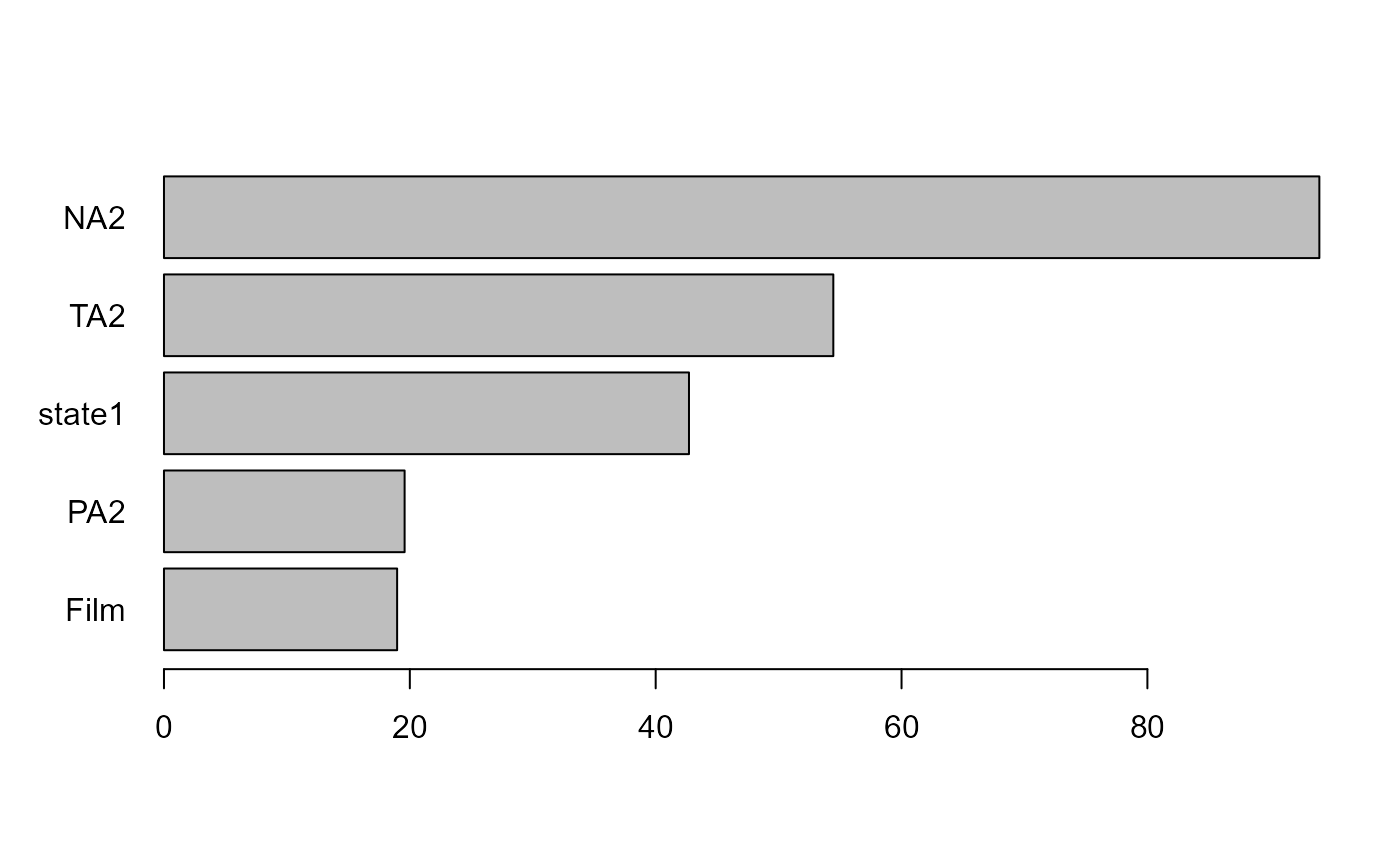

From this, we can learn that variables such as NA2 representing negative affect (after the movie), TA2 representing tense arousal (after the movie), and state1 representing the state anxiety before having watched the movie, are the best predictors of difference in the distribution of state anxiety (in either mean, variance or both) after having watched the movie.

Variable importance estimates are averaged across all trees by taking the mean importance of each variable over all trees. Sometimes, these estimates may be distorted if a single tree produces unstable estimates. To obtain a more robust estimate, it may make sense to take the median across all trees to obtain the variable importance estimates:

print(vim, sort.values=TRUE, aggregate="median")
#> Variable Importance
#>      Film       PA2    state1       TA2       NA2 
#>  7.539784 14.847694 39.679982 48.626777 73.758051
plot(vim, aggregate="median")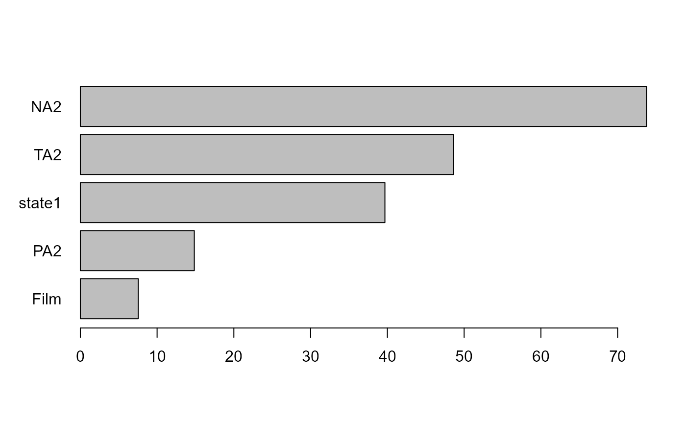

To inspect, how well these estimates converged, we can look at the convergence plot that shows the estimates as a function of the number of trees considered:

plot(vim, convergence=TRUE)

#> NULL

Partial Dependence

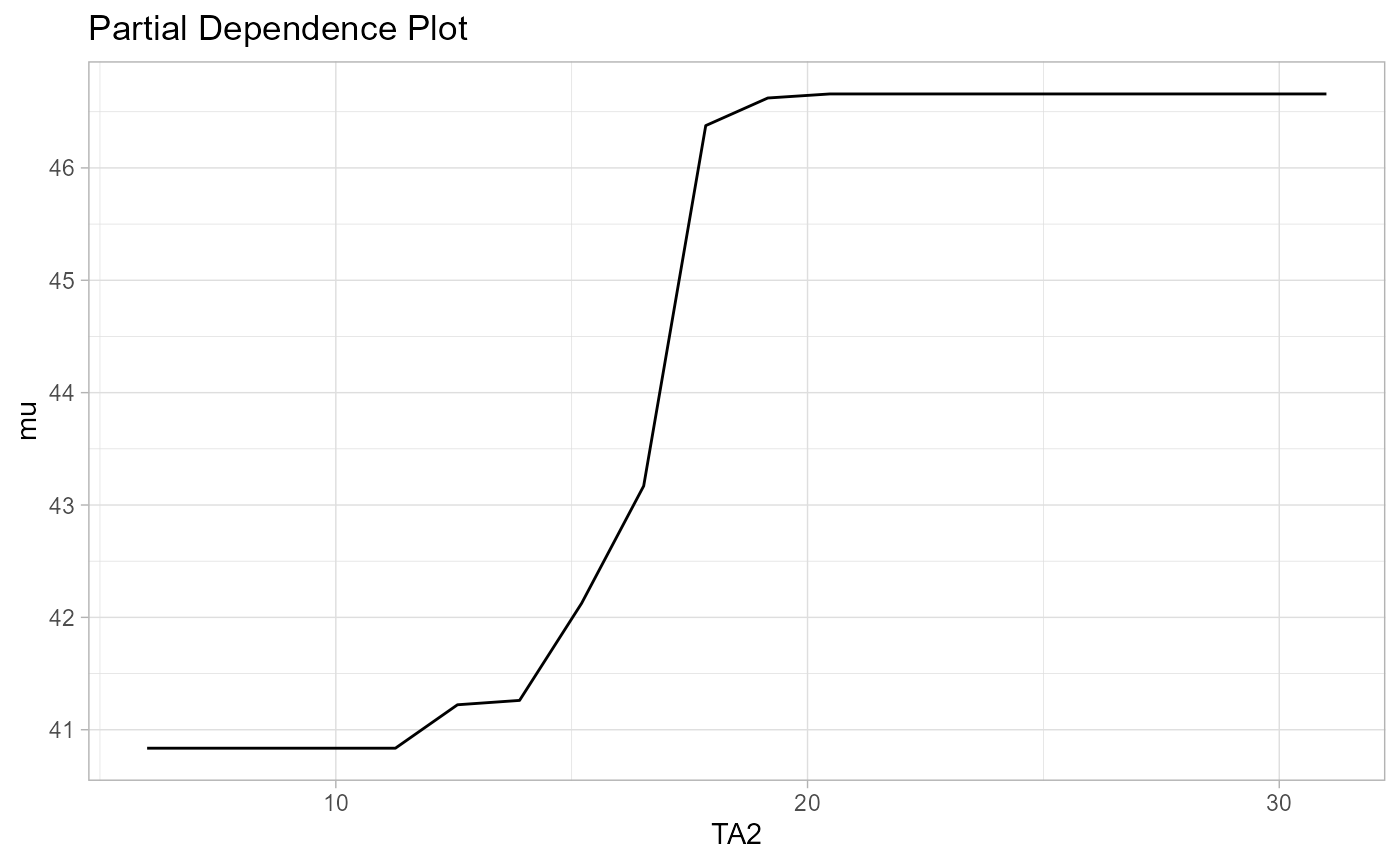
Partial dependence plots visualize the relationship of a predictor and a selected model parameter. This is a powerful tool to help with interpreting SEM forests.

pdp <- partialDependence(forest,reference.var = "TA2")

plot(pdp, parameter="mu")

Andreas Brandmaier

2026-01-23

Load data

Create simple model of state anxiety

Forest

Variable importance

Partial Dependence