summary(aov(sexism ~ factor(protest), psych::Garcia)) Df Sum Sq Mean Sq F value Pr(>F)
factor(protest) 2 1.08 0.5382 0.874 0.42
Residuals 126 77.55 0.6155 Analysis of Variance (ANOVA) is a test of differences in the means of a normally distributed variable across groups. We can implement this in a SEM in Onyx by representing each group with an observed variable representing the normal distribution in that group; that is, each variable needs a variance and a mean parameter. A grouping indicator (see Chapter: Multi-group models) can be used to assign each variable to a group. By cloning this model, wen can generate a model representing a null hypothesis (e.g., of equal means across groups) and perform a likelihood-ratio test (see Chapter: Model comparison) to make a statistical decision.
We use the dataset from the sexism protest study by Garcia et al. (2010). From the description of the dataset in the psych R package:
Garcia, Schmitt, Branscombe, and Ellemers (2010) report data for 129 subjects on the effects of perceived sexism on anger and liking of women’s reactions to ingroup members who protest discrimination.
[…]
A data frame with 129 observations on the following 6 variables.
protest0 = no protest, 1 = Individual Protest, 2 = Collective Protest
sexismMeans of an 8 item Modern Sexism Scale.
angerAnger towards the target of discrimination. “I feel angry towards Catherine”.
[…]
The reaction of women to women who protest discriminatory treatment was examined in an experiment reported by Garcia et al. (2010). 129 women were given a description of sex discrimination in the workplace (a male lawyer was promoted over a clearly more qualified female lawyer). Subjects then read that the target lawyer felt that the decision was unfair. Subjects were then randomly assigned to three conditions: Control (no protest), Individual Protest (“They are treating me unfairly”) , or Collective Protest (“The firm is is treating women unfairly”).
Participants were then asked how much they liked the target (liking), how angry they were to the target (anger) and to evaluate the appropriateness of the target’s response (respappr).
Load the dataset Garcia.csv
Specify an observed-only ANOVA model with three groups to test whether the sexism ratings differed across the three experimental (protest) groups.
Specify a null model, in which there are no mean differences
Use model comparison to decide between those models; is there a significant difference between groups?
Compare your results to ANOVA results from a different program (e.g., R or JASP); what is the difference?
Should variances be set equal across groups or not? What choice is most similar to classic ANOVA?
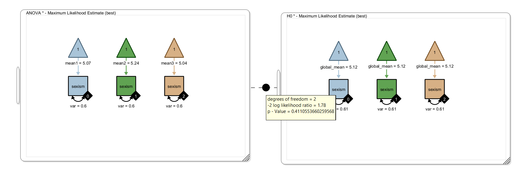
We specify a model with three copies of the outcome variable that each have a different grouping indicator to filter out only the cases of the respective group. Since group was coded 0,1, and 2, these are the values of the grouping indicators. Each variable has a mean (path from the triangle) and a variance. The variances are assumed to be identical (homoscedasticity assumption in ANOVA). We compare against a null model in which all means are assumed to be equal
summary(aov(sexism ~ factor(protest), psych::Garcia)) Df Sum Sq Mean Sq F value Pr(>F)
factor(protest) 2 1.08 0.5382 0.874 0.42
Residuals 126 77.55 0.6155 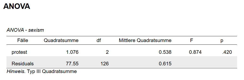
R and JASP both perform a classic ANOVA assuming normality within the groups and equality of variances across the groups. They both compute the exact F-statistic.
In the SEM solution presented here, we also assume normality within groups and equality of variances (even though it is easy to remove this constraint). Onyx computes an asymptotic Chi-Square-statistic. That is, asymptotically the results are the same but may differ in small to moderate sample sizes.
All three approaches yield a non-significant result, that is, there is no evidence that sexism ratings differed across protest groups.
  id    lhs op    rhs user block group free ustart exo label plabel start   est
1  1 sexism ~~ sexism    1     1     1    1     NA   0   var   .p1. 0.328 0.601
2  2 sexism ~1           1     1     1    2     NA   0         .p2. 5.037 5.037
3  3 sexism ~~ sexism    1     2     2    3     NA   0   var   .p3. 0.287 0.601
4  4 sexism ~1           1     2     2    4     NA   0         .p4. 5.071 5.071
5  5 sexism ~~ sexism    1     3     3    5     NA   0   var   .p5. 0.285 0.601
6  6 sexism ~1           1     3     3    6     NA   0         .p6. 5.245 5.245
7  7   .p1. ==   .p3.    2     0     0    0     NA   0              0.000 0.000
8  8   .p1. ==   .p5.    2     0     0    0     NA   0              0.000 0.000
     se
1 0.075
2 0.116
3 0.075
4 0.121
5 0.075
6 0.118
7 0.000
8 0.000
id lhs op rhs user block group free ustart exo label plabel start
1 1 sexism ~~ sexism 1 1 1 1 NA 0 var .p1. 0.328
2 2 sexism ~1 1 1 1 2 NA 0 m .p2. 5.037
3 3 sexism ~~ sexism 1 2 2 3 NA 0 var .p3. 0.287
4 4 sexism ~1 1 2 2 4 NA 0 m .p4. 5.071
5 5 sexism ~~ sexism 1 3 3 5 NA 0 var .p5. 0.285
6 6 sexism ~1 1 3 3 6 NA 0 m .p6. 5.245
7 7 .p1. == .p3. 2 0 0 0 NA 0 0.000
8 8 .p1. == .p5. 2 0 0 0 NA 0 0.000
9 9 .p2. == .p4. 2 0 0 0 NA 0 0.000
10 10 .p2. == .p6. 2 0 0 0 NA 0 0.000
est se
1 0.610 0.076
2 5.117 0.069
3 0.610 0.076
4 5.117 0.069
5 0.610 0.076
6 5.117 0.069
7 0.000 0.000
8 0.000 0.000
9 0.000 0.000
10 0.000 0.000 npar fmin chisq
4.000 0.001 0.284
df pvalue baseline.chisq
2.000 0.868 0.000
baseline.df baseline.pvalue cfi
0.000 NA 1.000
tli nnfi rfi
1.000 1.000 NA
nfi pnfi ifi
NA NA 1.000
rni logl unrestricted.logl
NA -150.221 -150.079
aic bic ntotal
308.442 319.882 129.000
bic2 rmsea rmsea.ci.lower
307.231 0.000 0.000
rmsea.ci.upper rmsea.ci.level rmsea.pvalue
0.156 0.900 0.880
rmsea.close.h0 rmsea.notclose.pvalue rmsea.notclose.h0
0.050 0.102 0.080
rmr rmr_nomean srmr
0.027 0.038 0.045
srmr_bentler srmr_bentler_nomean crmr
0.045 0.063 0.000
crmr_nomean srmr_mplus srmr_mplus_nomean
NaN 0.154 0.063
cn_05 cn_01 gfi
2724.629 4187.881 1.000
agfi pgfi mfi
1.000 0.333 1.007
ecvi
0.064 npar fmin chisq
2.000 0.008 2.062
df pvalue baseline.chisq
4.000 0.724 0.000
baseline.df baseline.pvalue cfi
0.000 NA 1.000
tli nnfi rfi
1.000 1.000 NA
nfi pnfi ifi
NA NA 1.000
rni logl unrestricted.logl
NA -151.110 -150.079
aic bic ntotal
306.220 311.940 129.000
bic2 rmsea rmsea.ci.lower
305.615 0.000 0.000
rmsea.ci.upper rmsea.ci.level rmsea.pvalue
0.167 0.900 0.762
rmsea.close.h0 rmsea.notclose.pvalue rmsea.notclose.h0
0.050 0.188 0.080
rmr rmr_nomean srmr
0.067 0.041 0.093
srmr_bentler srmr_bentler_nomean crmr
0.093 0.068 0.110
crmr_nomean srmr_mplus srmr_mplus_nomean
NaN 0.214 0.068
cn_05 cn_01 gfi
594.607 831.667 1.000
agfi pgfi mfi
0.999 0.666 1.008
ecvi
0.047
Chi-Squared Difference Test

      Df    AIC    BIC  Chisq Chisq diff RMSEA Df diff Pr(>Chisq)
mod    2 308.44 319.88 0.2838
modh0  4 306.22 311.94 2.0618      1.778     0       2     0.4111