Syntax Export
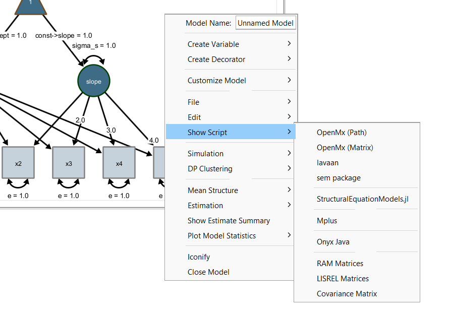
Onyx supports exports of models to syntax specifications of other languages. This way, Onyx can be used for graphical model specification and other programs can then be used if their more advanced features are needed for estimating models (e.g., other estimators or non-normally distributed variables, etc.). To view model syntax, right-click a model and choose “Show Script” and select a syntax of your choice. Importantly, this includes the widely used R packages OpenMx and lavaan but also commercial software such as Mplus:
Importantly, the model syntax view remains linked to the model, that is, if the model graph is changed (e.g., by adding or removing variables or paths in the path diagram), the model syntax is updated. Onyx highlights newly added code parts in yellow.
Exercise
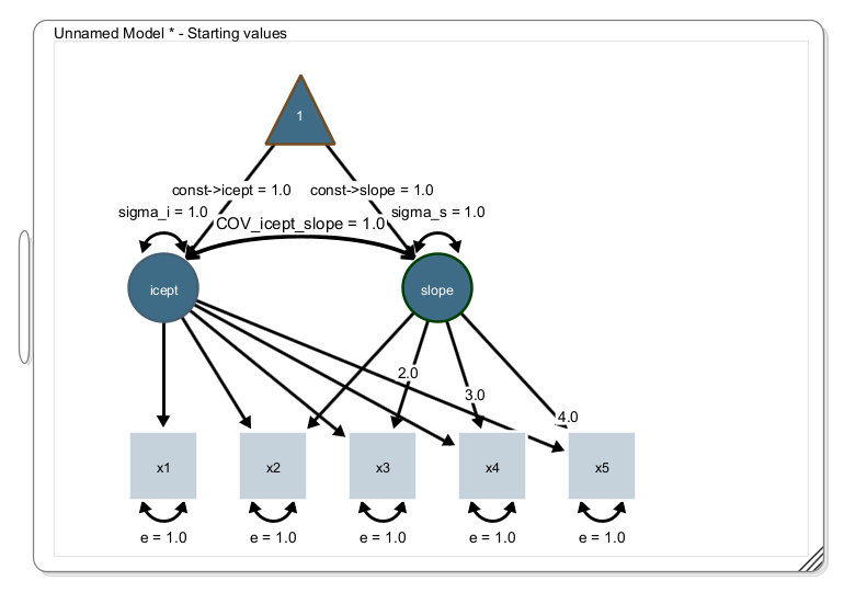
Create a linear latent growth curve model using the linear latent growth curve model wizard (right-click the desktop, select “Create new model -> Create new LGCM”; make sure to estimate a covariance between intercept and slope (click the respective option in the dialog)
Don’t forget to use some of the visual options to change the appearance of the diagram
Load the data “lgcm_simulated.csv” and obtain parameter estimates; inspect model fit
Open the model syntax view for lavaan
If you are familiar with lavaan and R: Copy the lavaan code to an R session; adapt the code to load the data file; estimate the model in lavaan; compare the results between Onyx and lavaan
Solution
The path diagram should look like this (showing the starting values; not the parameter estimates):
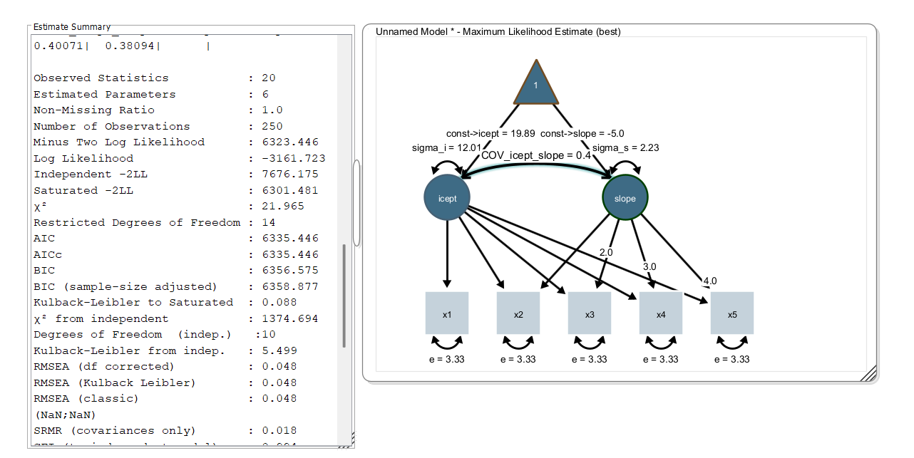
Load the dataset, select all variables, right-click on the data view and click “send data to model”. Model estimation starts and your parameter estimates and model fit statistics should look like this:
 This is the lavaan model syntax as generated by Onyx:
#
# This model specification was automatically generated by Onyx
#
library(lavaan);
modelData <- read.table(DATAFILENAME, header = TRUE) ;
 model<-"
   ! regressions
   icept=~1.0*x1
   icept=~1.0*x2
   slope=~1.0*x2
   icept=~1.0*x3
   slope=~2.0*x3
   icept=~1.0*x4
   slope=~3.0*x4
   icept=~1.0*x5
   slope=~4.0*x5
   ! residuals, variances and covariances
   x1 ~~ e*x1
   x2 ~~ e*x2
   x3 ~~ e*x3
   x4 ~~ e*x4
   x5 ~~ e*x5
   icept ~~ sigma_i*icept
   slope ~~ sigma_s*slope
   icept ~~ COV_icept_slope*slope
   ! means
   icept ~ const__icept*1
   slope ~ const__slope*1
   x1 ~ 0.0*1
   x2 ~ 0.0*1
   x3 ~ 0.0*1
   x4 ~ 0.0*1
   x5 ~ 0.0*1
"
result<-lavaan(model, data=modelData, fixed.x=FALSE, missing="FIML")
summary(result, fit.measures=TRUE)
In this code, you only need to replace the placeholder “DATAFILENAME” with the path to a data file on your computer. Then, model estimation in R using the lavaan package yields:
Warning: Paket 'lavaan' wurde unter R Version 4.5.3 erstellt
This is lavaan 0.6-21
lavaan is FREE software! Please report any bugs.
lavaan 0.6-21 ended normally after 52 iterations

  Estimator                                         ML
  Optimization method                           NLMINB
  Number of model parameters                        10
  Number of equality constraints                     4

  Number of observations                           250
  Number of missing patterns                         1

Model Test User Model:

  Test statistic                                21.965
  Degrees of freedom                                14
  P-value (Chi-square)                           0.079

Model Test Baseline Model:

  Test statistic                              1374.694
  Degrees of freedom                                10
  P-value                                        0.000

User Model versus Baseline Model:

  Comparative Fit Index (CFI)                    0.994
  Tucker-Lewis Index (TLI)                       0.996

  Robust Comparative Fit Index (CFI)             0.994
  Robust Tucker-Lewis Index (TLI)                0.996

Loglikelihood and Information Criteria:

  Loglikelihood user model (H0)              -3161.723
  Loglikelihood unrestricted model (H1)      -3150.741

  Akaike (AIC)                                6335.446
  Bayesian (BIC)                              6356.575
  Sample-size adjusted Bayesian (SABIC)       6337.554

Root Mean Square Error of Approximation:

  RMSEA                                          0.048
  90 Percent confidence interval - lower         0.000
  90 Percent confidence interval - upper         0.084
  P-value H_0: RMSEA <= 0.050                    0.497
  P-value H_0: RMSEA >= 0.080                    0.076

  Robust RMSEA                                   0.048
  90 Percent confidence interval - lower         0.000
  90 Percent confidence interval - upper         0.084
  P-value H_0: Robust RMSEA <= 0.050             0.497
  P-value H_0: Robust RMSEA >= 0.080             0.076

Standardized Root Mean Square Residual:

  SRMR                                           0.014

Parameter Estimates:

  Standard errors                             Standard
  Information                                 Observed
  Observed information based on                Hessian

Latent Variables:
                   Estimate  Std.Err  z-value  P(>|z|)
  icept =~
    x1                1.000
    x2                1.000
  slope =~
    x2                1.000
  icept =~
    x3                1.000
  slope =~
    x3                2.000
  icept =~
    x4                1.000
  slope =~
    x4                3.000
  icept =~
    x5                1.000
  slope =~
    x5                4.000

Covariances:
                   Estimate  Std.Err  z-value  P(>|z|)
  icept ~~
    slope   (COV_)    0.401    0.381    1.052    0.293

Intercepts:
                   Estimate  Std.Err  z-value  P(>|z|)
    icpt (cnst__c)   19.889    0.237   84.022    0.000
    slop (cnst__s)   -4.999    0.101  -49.371    0.000
   .x1                0.000
   .x2                0.000
   .x3                0.000
   .x4                0.000
   .x5                0.000

Variances:
                   Estimate  Std.Err  z-value  P(>|z|)
   .x1         (e)    3.335    0.172   19.365    0.000
   .x2         (e)    3.335    0.172   19.365    0.000
   .x3         (e)    3.335    0.172   19.365    0.000
   .x4         (e)    3.335    0.172   19.365    0.000
   .x5         (e)    3.335    0.172   19.365    0.000
    icept  (sigm_)   12.007    1.257    9.551    0.000
    slope  (sgm_s)    2.230    0.230    9.699    0.000
As you can see, all parameter estimates and fit statistics are identical.